Reflekt Lab - Building Smarter Context: Search Strategies That Make AI Actually Useful

AI models are powerful, but they're only as good as the context you give them. Ask a model to categorize a transaction or match a product without reference examples, and you'll get confident-sounding garbage. Give it the right 10–15 examples from your own data, and accuracy jumps from "demo-grade" to "production-grade."

The hard part isn't the AI call — it's finding the right context to feed it.

We run several production pipelines — product matching, transaction categorization, inventory mapping — each pulling context from spreadsheets and external services. Over time, a clear pattern emerged: no single search strategy is good enough, but combining them hides each method's weaknesses while stacking their strengths.

This post breaks down the three search strategies we use, where each one fails, and why overlapping them works.

The Pattern: Search → Merge → Reason → Validate

Every context-enriched AI pipeline follows the same shape:

Input → Parallel search (multiple strategies) → Deduplicate & rank → AI reasoning with context → Validate output

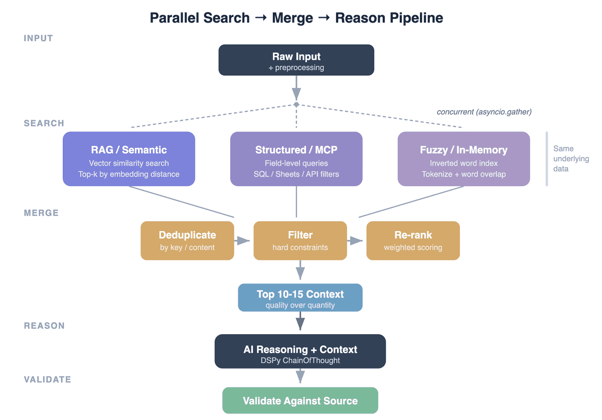
The interesting part is the search layer. Each strategy has a fundamentally different failure mode — and that's exactly why combining them works.

RAG (Retrieval-Augmented Generation) Semantic Search: Understands Meaning, Loses Precision

How it works: Your reference data is chunked into text, embedded into vectors, and stored in a vector database. At query time, the input is embedded and the nearest neighbors are returned by cosine similarity.

Where it shines:

Paraphrased or reformulated inputs. "VIR SEPA LEASYS FRANCE SAS LOYER" and "VIREMENT LEASYS — LEASE MENSUEL" are distant in keyword space but close in embedding space.
Longer, descriptive queries where the embedding model captures overall meaning well.
Discovery — finding relevant records you didn't know to search for by keyword.

Where it fails:

Exact identifiers. Embeddings blur the difference between "61350000" and "61360000" — they're both 8-digit codes, semantically identical to the model. If your task depends on exact code matching, RAG will sometimes return the wrong one.
Structurally similar but semantically different names. "St Emilion" and "St Estephe" share the same prefix and shape — embeddings often score them closer to each other than "St Emilion" and "Saint-Émilion," which are actually the same place. The model sees surface pattern similarity, not domain knowledge. This is a common trap: short names with shared structure confuse vector search.
Structured field matching. When you need "Winery = X AND Region = Y", semantic similarity doesn't respect field boundaries. A record with the right winery but wrong region can score higher than the exact match.
Short, cryptic inputs. Bank codes, SKUs, or abbreviated product names don't embed well — there's not enough semantic signal.

Data source fit:

Works well over any text-heavy data: spreadsheet rows serialized to strings, database records flattened to text, document chunks, log entries.
Equally applicable to PostgreSQL full-text, Elasticsearch, or a dedicated vector DB — the pattern is the same regardless of where the raw data lives.

MCP (Model Context Protocol) / Structured Search: Precise Lookups, Brittle to Variation

How it works: A structured query against your data source — Google Sheets via MCP tools, a SQL query against a database, an API call to a search service. The query is parsed from the input (extract entity names, filter by type) and executed as a direct lookup.

Where it shines:

Exact field matching. "Give me all products where Winery = 'Domaine Faiveley'" returns exactly that — no fuzzy nonsense.
Filtered search. Combining multiple constraints (type + region + name) narrows results to precisely relevant records.
Deterministic results. Same query always returns the same results. No embedding drift, no model version sensitivity.

Where it fails:

Typos and abbreviations. Search for "Chateau Latour" when the record says "Château Latour" — accent mismatch, zero results. Search for "Dom. Faiveley" when the record says "Domaine Faiveley" — no match.
Reformulations. The user writes "red wine from Burgundy"; the database field says "Bourgogne." Structured search has no concept of synonymy.
Schema coupling. Every new data source needs query logic tailored to its schema. Move from Google Sheets to PostgreSQL and the search code changes, even though the pattern is identical.

Data source fit:

Natural fit for databases (SQL WHERE clauses), Google Sheets (column-based filtering via MCP), REST APIs with filter parameters.
This can be abstracted behind MCP tools — the LLM pipeline doesn't need to know whether the backend is Sheets, Postgres, or Salesforce; the MCP server handles the translation.

Fuzzy / In-Memory Search: Catches Partial Matches, Noisy at Scale

How it works: Build an inverted word index from your reference data at startup. At query time, tokenize the input, remove stop words, and score records by word overlap. Optionally add edit-distance matching for typo tolerance.

Where it shines:

Partial matches across fields. Input "Bourgogne Pinot Noir Faiveley 2020" matches a record where "Bourgogne" is in the region field, "Pinot Noir" is in the grape field, and "Faiveley" is in the winery field. Neither RAG (which embeds the whole string) nor structured search (which queries one field at a time) handles this well.
Compound descriptions. Real-world inputs often contain information from multiple schema fields mashed together. Word-level overlap naturally bridges this gap.
Zero infrastructure. No vector DB, no search service — just an in-memory dict built at startup. Often millisecond latency for selective indexed lookups.

Where it fails:

Scale. Works great for thousands of records. At millions, the inverted index gets large and scoring becomes expensive. At that point, you need a proper search engine.
Semantic gaps. "Leasing payment" and "LOYER MENSUEL" share zero words. Fuzzy search won't connect them.
Noise at low overlap. A single matching word can surface irrelevant records. Without a minimum overlap threshold, results degrade quickly.

Data source fit:

Best for datasets small enough to hold in memory (up to low hundreds of thousands of records).
Works identically regardless of source — load from a spreadsheet, a database dump, a CSV, or an API response. The index is built in-process.

Why Overlapping Works: Failure Modes Don't Correlate

The key insight: these three strategies fail on different inputs.

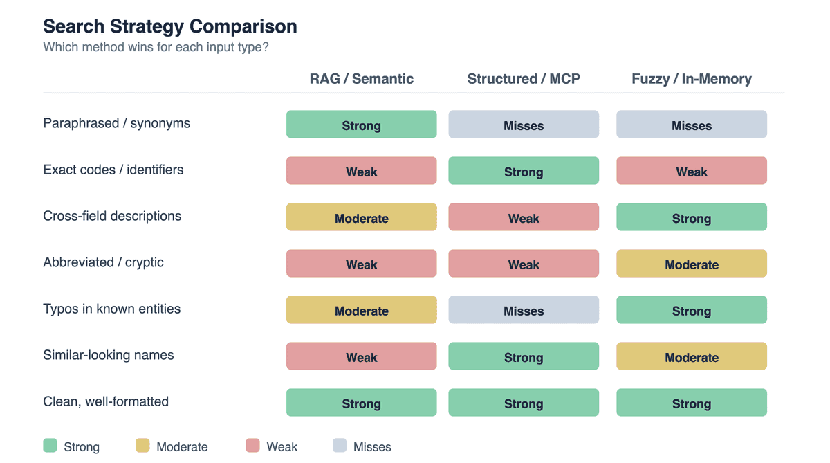
When you run all three in parallel and merge results, the winning strategy is almost always present for any given input. The merge-and-rank layer just needs to surface it.

The cost of overlap is low:

Each additional search adds milliseconds (they run concurrently).
Deduplication removes redundant results before they reach the AI model.
The model doesn't care which strategy found the context — it just needs the right examples.

The Merge Layer: Deduplication, Filtering, Re-Ranking

Running three searches produces redundant, sometimes contradictory results. The merge layer is critical:

Deduplication: Same record found by multiple strategies → keep one. We deduplicate by normalized content (lowercase, whitespace-collapsed). For database-backed sources, deduplication by primary key is even more reliable.

Filtering: Remove results that violate hard constraints. If the input specifies "Type = Red Wine," drop any White Wine results regardless of search score. This is where domain logic lives.

Re-ranking: Score remaining results by relevance to the original input. We use weighted word overlap (different weights per field — entity names matter more than categories). This re-ranking corrects for differences in scoring semantics across search backends.

Context cap: Limit the final context to 10–15 entries. We tested uncapped context and found that beyond ~15 examples, the AI starts "averaging" across all examples rather than identifying the best match. Fewer, more relevant examples consistently outperform many mediocre ones.

Pre-Processing: Context Quality Starts Before Search

Search quality depends on input cleaning. Before any search runs:

Expand abbreviations deterministically (domain-specific shorthand → full form). This fixes RAG's blind spot on cryptic inputs.
Normalize encoding (accents, unicode, case). This fixes structured search's brittleness to variation.
Remove noise tokens (size codes, format prefixes, boilerplate). This improves fuzzy search precision by reducing false word overlaps.
Early returns for trivially resolvable inputs (known patterns that don't need LLM reasoning).

Pre-processing is invisible to the AI but often makes a bigger accuracy difference than switching models.

Post-AI Validation: Trust but Verify

Context-enriched AI outputs are better, but not perfect. Validation patterns:

Category validation: Check predicted categories against the known valid set. Flag or reject unknowns.
Progressive key matching: Try exact match against reference data, then progressively relax constraints (drop optional fields) until a match is found or confidence drops below threshold.
Output-input consistency check: Verify that distinctive terms from the input appear in the output. If the model hallucinated a different entity, fall back to the highest-scoring search result.

A Different Pattern: Agentic Search for Interactive Use

The parallel search pipeline described above is designed for batch processing — hundreds or thousands of items processed consistently, without human involvement. Same input always triggers the same search strategies, same merge logic, same validation. It's deterministic, repeatable, and optimized for throughput.

But not every use case is batch. Our CRM assistant takes a fundamentally different approach, designed for interactive, one-at-a-time requests from a user.

The CRM pipeline processes natural language requests — "how is Marcelo doing?" or "create a contact at TechCorp" — through a ReAct (Reasoning + Acting) agent. Instead of pre-gathering context and reasoning once, the AI decides what to search for, iteratively, calling MCP tools against a PostgreSQL-backed CRM:

Request → LLM chooses tool → MCP executes query → LLM reads result → LLM acts or responds (up to 5 iterations)

The MCP server exposes multiple different tools (SQL filters by name, status, lifecycle, priority), plus write operations with dry-run support. Smaller lists like batches and tags use in-memory substring matching.

Why this works for interactive use but not for batch:

One user, one question at a time. The AI can spend multiple iterations refining its search — if a query returns nothing, the ReAct agent tries different parameters or a broader query. Affordable for a single request; prohibitively expensive at scale.
CRM data is well-structured. Contacts have names, companies, statuses, stages. Users search by these fields — not by semantic similarity. Structured search alone covers the query space.
Latency tolerance is higher. A user waiting 2–3 seconds for a CRM answer is fine. Processing 500 inventory rows at 2–3 seconds each with multiple LLM calls per row is not.

The heuristic: use agentic search for interactive, user-facing queries where the AI can iterate and the data model is clean. Use parallel pre-gathered context for batch processing — where you need consistency (same search for every item), throughput (concurrent searches, one AI call per item), and debuggability (search diagnostics tell you exactly which strategy contributed what).

Applying Beyond Spreadsheets: Databases, APIs, and Beyond

But the pattern is data-source agnostic:

Relational databases (PostgreSQL, MySQL):

Structured search → SQL queries with WHERE clauses, parameterized by parsed input fields. Indexes on frequently queried columns often make this sub-millisecond under light workloads.
RAG → Embed table rows as text (concatenate relevant columns), index in pgvector or a sidecar vector DB. Same semantic search, backed by your existing database.
Fuzzy → pg_trgm extension for trigram-based fuzzy matching, or ILIKE with wildcards. Alternatively, load a working set into memory at startup for word-overlap scoring.

Document stores (MongoDB, Elasticsearch):

Structured search → Elasticsearch term/match queries. MongoDB $text search or regex queries.
RAG → Elasticsearch dense vector fields with kNN search, or MongoDB Atlas Vector Search. Both support hybrid keyword+vector queries natively.
Fuzzy → Elasticsearch's fuzziness parameter on match queries. MongoDB $regex for simple patterns.

External APIs (CRM, ERP, SaaS):

Structured search → API filter parameters. Most SaaS APIs support field-specific search.
RAG → Periodic sync: pull records, embed, index. Search the local vector index, return matching records with their API IDs.
Fuzzy → Depends on API capabilities. Many offer built-in fuzzy search; if not, sync and build a local index.

The abstraction layer (MCP in our case) makes this practical. The AI pipeline calls "search for similar records" — the MCP server translates that to the appropriate backend query. Swap Google Sheets for PostgreSQL, and only the MCP tool implementation changes.

What We Learned

Overlapping strategies beat optimizing a single one. Each search method has structural blind spots. Running all three and merging results is simpler and more robust than perfecting any single approach.
Context quality > context quantity. 15 well-chosen examples beat 50 mediocre ones. Deduplication, filtering, and re-ranking matter more than retrieval volume.
Pre-processing is half the battle. Abbreviation expansion and normalization before search often make a bigger accuracy difference than switching models.
Choose your pattern by workload. Batch processing needs deterministic parallel search. Interactive use cases can afford agentic iteration. Don't force one pattern on both.

The Bottom Line

The AI model is the easy part. The search infrastructure that feeds it determines whether your system works in production. Semantic search, structured lookup, and fuzzy matching each cover different failure modes. Overlap them, deduplicate, rank — and the AI gets context good enough to reason correctly.

If your AI pipeline is underperforming, look at the context first. Chances are the model is fine — it just can't see what it needs.

For more on our production LLM setup, check out our model benchmarks and vision-based document processing.